Pandas#
Pandas是基于Numpy创建的Python库,为Python提供了易于使用的数据结构和数据分析工具。
使用以下语句导入Pandas库:
import pandas as pd
Pandas数据结构#
Series - 序列#
存储任意类型数据的一维数组
s = pd.Series([3, -5, 7, 4], index=["a", "b", "c", "d"])
DataFrame - 数据帧#
data = {
    "Country": ["Belgium", "India", "Brazil"],
    "Capital": ["Brussels", "New Delhi", "Brasília"],
    "Population": [11190846, 1303171035, 207847528],
}
df = pd.DataFrame(data, columns=["Country", "Capital", "Population"])
df
| Country | Capital | Population | |
|---|---|---|---|
| 0 | Belgium | Brussels | 11190846 |
| 1 | India | New Delhi | 1303171035 |
| 2 | Brazil | Brasília | 207847528 |
输入/输出#
读取/写入CSV#
df.to_csv("../_tmp/df_to_csv.csv", index=False)
pd.read_csv("../_tmp/df_to_csv.csv", nrows=5)
| Country | Capital | Population | |
|---|---|---|---|
| 0 | Belgium | Brussels | 11190846 |
| 1 | India | New Delhi | 1303171035 |
| 2 | Brazil | Brasília | 207847528 |
读取/写入Excel#
df.to_excel("../_tmp/df_to_excel.xlsx", index=False, sheet_name="Sheet1")
pd.read_excel("../_tmp/df_to_excel.xlsx")
| Country | Capital | Population | |
|---|---|---|---|
| 0 | Belgium | Brussels | 11190846 |
| 1 | India | New Delhi | 1303171035 |
| 2 | Brazil | Brasília | 207847528 |
xlsx = pd.ExcelFile("../_tmp/df_to_excel.xlsx") # 读取内含多个表的 Excel
df = pd.read_excel(xlsx, "Sheet1") # 读取多表 Excel 中的 Sheet1 表
df
| Country | Capital | Population | |
|---|---|---|---|
| 0 | Belgium | Brussels | 11190846 |
| 1 | India | New Delhi | 1303171035 |
| 2 | Brazil | Brasília | 207847528 |
筛选数据#
取值#
s["b"] # 取序列的值
np.int64(-5)
df[1:] # 取数据帧的子集
| Country | Capital | Population | |
|---|---|---|---|
| 1 | India | New Delhi | 1303171035 |
| 2 | Brazil | Brasília | 207847528 |
选取、布尔索引及设置值#
按位置
df.iloc[[0], [0]] # 按行与列的位置选择某值
| Country | |
|---|---|
| 0 | Belgium |
df.iat[0, 0]
'Belgium'
按标签
df.loc[[0], ["Country"]] # 按行与列的名称选择某值
| Country | |
|---|---|
| 0 | Belgium |
df.at[0, "Country"] # 按行与列的名称选择某值
'Belgium'
按标签/位置
df.loc[2] # 选择某行
Country          Brazil
Capital        Brasília
Population    207847528
Name: 2, dtype: object
df.loc[:, "Capital"] # 选择某列
0     Brussels
1    New Delhi
2     Brasília
Name: Capital, dtype: object
df.loc[1, "Capital"] # 按行列取值
'New Delhi'
布尔索引
s[~(s > 1)] # 序列 S 中没有大于 1 的值
b   -5
dtype: int64
s[(s < -1) | (s > 2)] # 序列 S 中小于 -1 或大于 2 的值
a    3
b   -5
c    7
d    4
dtype: int64
df[df["Population"] > 1200000000] # 选择数据帧中 Population 大于 12 亿的数据
| Country | Capital | Population | |
|---|---|---|---|
| 1 | India | New Delhi | 1303171035 |
df.loc[
    df["Population"] > 1200000000, ["Country", "Capital"]
]  # 选择数据帧中人口大于 12 亿的数据 'Country' 和 'Capital' 字段
| Country | Capital | |
|---|---|---|
| 1 | India | New Delhi |
设置值
s["a"] = 6 # 将序列 s 中索引为 a 的值设为 6
删除数据#
通过drop函数删除数据
s.drop(["a", "c"]) # 按索引删除序列的值 (axis=0)
b   -5
d    4
dtype: int64
df.drop("Country", axis=1) # 按列名删除数据帧的列 (axis=1)
| Capital | Population | |
|---|---|---|
| 0 | Brussels | 11190846 |
| 1 | New Delhi | 1303171035 |
| 2 | Brasília | 207847528 |
排序和排名#
根据索引或者值进行排序
df.sort_index() # 按索引排序
| Country | Capital | Population | |
|---|---|---|---|
| 0 | Belgium | Brussels | 11190846 |
| 1 | India | New Delhi | 1303171035 |
| 2 | Brazil | Brasília | 207847528 |
df.sort_values(by="Country") # 按某列的值排序
| Country | Capital | Population | |
|---|---|---|---|
| 0 | Belgium | Brussels | 11190846 |
| 2 | Brazil | Brasília | 207847528 |
| 1 | India | New Delhi | 1303171035 |
df.rank() # 数据帧排名
| Country | Capital | Population | |
|---|---|---|---|
| 0 | 1.0 | 2.0 | 1.0 |
| 1 | 3.0 | 3.0 | 3.0 |
| 2 | 2.0 | 1.0 | 2.0 |
查询信息与计算#
基本信息#
df.shape # (行,列)
(3, 3)
df.index # 获取索引
RangeIndex(start=0, stop=3, step=1)
df.columns # 获取列名
Index(['Country', 'Capital', 'Population'], dtype='object')
df.info() # 获取数据帧基本信息
<class 'pandas.core.frame.DataFrame'>
RangeIndex: 3 entries, 0 to 2
Data columns (total 3 columns):
 #   Column      Non-Null Count  Dtype
---  ------      --------------  -----
 0   Country     3 non-null      object
 1   Capital     3 non-null      object
 2   Population  3 non-null      int64
dtypes: int64(1), object(2)
memory usage: 204.0+ bytes
df.count() # 非 Na 值的数量
Country       3
Capital       3
Population    3
dtype: int64
汇总#
df.sum() # 合计
Country              BelgiumIndiaBrazil
Capital       BrusselsNew DelhiBrasília
Population                   1522209409
dtype: object
df.cumsum() # 累计
| Country | Capital | Population | |
|---|---|---|---|
| 0 | Belgium | Brussels | 11190846 |
| 1 | BelgiumIndia | BrusselsNew Delhi | 1314361881 |
| 2 | BelgiumIndiaBrazil | BrusselsNew DelhiBrasília | 1522209409 |
df["Population"].min() / df["Population"].max() # 最小值除以最大值
np.float64(0.008587396204673933)
df["Population"].idxmin() / df["Population"].idxmax() # 索引最小值除以索引最大值
0.0
df.describe() # 基础统计数据
| Population | |
|---|---|
| count | 3.000000e+00 |
| mean | 5.074031e+08 |
| std | 6.961346e+08 |
| min | 1.119085e+07 |
| 25% | 1.095192e+08 |
| 50% | 2.078475e+08 |
| 75% | 7.555093e+08 |
| max | 1.303171e+09 |
df["Population"].mean() # 平均值
np.float64(507403136.3333333)
df["Population"].median() # 中位数
np.float64(207847528.0)
应用函数#
通过apply函数应用变换
f = lambda x: x * 2 # 应用匿名函数 lambda
df.apply(f) # 应用函数
| Country | Capital | Population | |
|---|---|---|---|
| 0 | BelgiumBelgium | BrusselsBrussels | 22381692 |
| 1 | IndiaIndia | New DelhiNew Delhi | 2606342070 |
| 2 | BrazilBrazil | BrasíliaBrasília | 415695056 |
df.applymap(f) # 对每个单元格应用函数
/tmp/ipykernel_2583/1512017809.py:1: FutureWarning: DataFrame.applymap has been deprecated. Use DataFrame.map instead.
  df.applymap(f)  # 对每个单元格应用函数
| Country | Capital | Population | |
|---|---|---|---|
| 0 | BelgiumBelgium | BrusselsBrussels | 22381692 |
| 1 | IndiaIndia | New DelhiNew Delhi | 2606342070 |
| 2 | BrazilBrazil | BrasíliaBrasília | 415695056 |
数据对齐#
内部数据对齐#
如有不一致的索引,则使用NA值:
s3 = pd.Series([7, -2, 3], index=["a", "c", "d"])
s + s3
a    13.0
b     NaN
c     5.0
d     7.0
dtype: float64
使用 Fill 方法运算#
还可以使用 Fill 方法补齐缺失后再运算:
s.add(s3, fill_value=0)
a    13.0
b    -5.0
c     5.0
d     7.0
dtype: float64
s.sub(s3, fill_value=2)
a   -1.0
b   -7.0
c    9.0
d    1.0
dtype: float64
s.div(s3, fill_value=4)
a    0.857143
b   -1.250000
c   -3.500000
d    1.333333
dtype: float64
s.mul(s3, fill_value=3)
a    42.0
b   -15.0
c   -14.0
d    12.0
dtype: float64
数据重塑#
import pandas as pd

df2 = pd.DataFrame(
    {
        "Date": [
            "2021-12-25",
            "2021-12-26",
            "2021-12-25",
            "2021-12-27",
            "2021-12-26",
            "2021-12-27",
        ],
        "Type": ["a", "b", "c", "a", "a", "c"],
        "Value": [1.34, 10.2, 20.43, 50.31, 0.26, 20.64],
    }
)
透视#
df3 = df2.pivot(index="Date", columns="Type", values="Value")  # 将行变为列
df3
| Type | a | b | c |
|---|---|---|---|
| Date | |||
| 2021-12-25 | 1.34 | NaN | 20.43 |
| 2021-12-26 | 0.26 | 10.2 | NaN |
| 2021-12-27 | 50.31 | NaN | 20.64 |
透视表#
df4 = pd.pivot_table(df2, values="Value", index="Date", columns="Type")  # 将行变为列
df4
| Type | a | b | c |
|---|---|---|---|
| Date | |||
| 2021-12-25 | 1.34 | NaN | 20.43 |
| 2021-12-26 | 0.26 | 10.2 | NaN |
| 2021-12-27 | 50.31 | NaN | 20.64 |
堆叠(轴旋转)#
stacked = df2.stack()  # 透视列标签
stacked
0  Date     2021-12-25
   Type              a
   Value          1.34
1  Date     2021-12-26
   Type              b
   Value          10.2
2  Date     2021-12-25
   Type              c
   Value         20.43
3  Date     2021-12-27
   Type              a
   Value         50.31
4  Date     2021-12-26
   Type              a
   Value          0.26
5  Date     2021-12-27
   Type              c
   Value         20.64
dtype: object
stacked.unstack() # 透视索引标签
| Date | Type | Value | |
|---|---|---|---|
| 0 | 2021-12-25 | a | 1.34 |
| 1 | 2021-12-26 | b | 10.2 |
| 2 | 2021-12-25 | c | 20.43 |
| 3 | 2021-12-27 | a | 50.31 |
| 4 | 2021-12-26 | a | 0.26 |
| 5 | 2021-12-27 | c | 20.64 |
融合/Melt#
pd.melt(
    df2, id_vars=["Date"], value_vars=["Type", "Value"], value_name="Observations"
)  # 将列转为行
| Date | variable | Observations | |
|---|---|---|---|
| 0 | 2021-12-25 | Type | a |
| 1 | 2021-12-26 | Type | b |
| 2 | 2021-12-25 | Type | c |
| 3 | 2021-12-27 | Type | a |
| 4 | 2021-12-26 | Type | a |
| 5 | 2021-12-27 | Type | c |
| 6 | 2021-12-25 | Value | 1.34 |
| 7 | 2021-12-26 | Value | 10.2 |
| 8 | 2021-12-25 | Value | 20.43 |
| 9 | 2021-12-27 | Value | 50.31 |
| 10 | 2021-12-26 | Value | 0.26 |
| 11 | 2021-12-27 | Value | 20.64 |
迭代#
迭代遍历数据帧
df2.items() # (列索引, 序列) 键值对
<generator object DataFrame.items at 0x737ebe713010>
df2.iterrows() # (行索引, 序列) 键值对
<generator object DataFrame.iterrows at 0x737ebe78c6a0>
高级索引#
基础选择
df3.loc[:, (df3 > 1).any()] # 选择任一值大于 1 的列
| Type | a | b | c |
|---|---|---|---|
| Date | |||
| 2021-12-25 | 1.34 | NaN | 20.43 |
| 2021-12-26 | 0.26 | 10.2 | NaN |
| 2021-12-27 | 50.31 | NaN | 20.64 |
df3.loc[:, (df3 > 1).all()] # 选择所有值大于 1 的列
| Type |
|---|
| Date |
| 2021-12-25 |
| 2021-12-26 |
| 2021-12-27 |
df3.loc[:, df3.isnull().any()] # 选择含 NaN 值的列
| Type | b | c |
|---|---|---|
| Date | ||
| 2021-12-25 | NaN | 20.43 |
| 2021-12-26 | 10.2 | NaN |
| 2021-12-27 | NaN | 20.64 |
df3.loc[:, df3.notnull().all()] # 选择不含 NaN 值的列
| Type | a |
|---|---|
| Date | |
| 2021-12-25 | 1.34 |
| 2021-12-26 | 0.26 |
| 2021-12-27 | 50.31 |
通过isin选择
df2[(df2.Type.isin(["b", "c"]))] # 选择指定列为某一类型的数值
| Date | Type | Value | |
|---|---|---|---|
| 1 | 2021-12-26 | b | 10.20 |
| 2 | 2021-12-25 | c | 20.43 |
| 5 | 2021-12-27 | c | 20.64 |
df3.filter(items=["a", "b"]) # 选择特定值
| a | b | |
|---|---|---|
| Date | ||
| 2021-12-25 | 1.34 | NaN |
| 2021-12-26 | 0.26 | 10.2 |
| 2021-12-27 | 50.31 | NaN |
通过where选择
s = pd.Series([-1, 3, -5, 7, 4])
s.where(s > 0)  # 选择子集
0    NaN
1    3.0
2    NaN
3    7.0
4    4.0
dtype: float64
通过query选择
df2.query("Value > 10") # 查询 DataFrame
| Date | Type | Value | |
|---|---|---|---|
| 1 | 2021-12-26 | b | 10.20 |
| 2 | 2021-12-25 | c | 20.43 |
| 3 | 2021-12-27 | a | 50.31 |
| 5 | 2021-12-27 | c | 20.64 |
设置/取消索引#
df2.set_index("Date") # 设置索引
| Type | Value | |
|---|---|---|
| Date | ||
| 2021-12-25 | a | 1.34 |
| 2021-12-26 | b | 10.20 |
| 2021-12-25 | c | 20.43 |
| 2021-12-27 | a | 50.31 |
| 2021-12-26 | a | 0.26 |
| 2021-12-27 | c | 20.64 |
df2.reset_index() # 重置索引 0 ~ n
| index | Date | Type | Value | |
|---|---|---|---|---|
| 0 | 0 | 2021-12-25 | a | 1.34 |
| 1 | 1 | 2021-12-26 | b | 10.20 |
| 2 | 2 | 2021-12-25 | c | 20.43 |
| 3 | 3 | 2021-12-27 | a | 50.31 |
| 4 | 4 | 2021-12-26 | a | 0.26 |
| 5 | 5 | 2021-12-27 | c | 20.64 |
df2.rename(
    index=str, columns={"Date": "Time", "Type": "Category", "Value": "Number"}
)  # 重命名 DataFrame 列名
| Time | Category | Number | |
|---|---|---|---|
| 0 | 2021-12-25 | a | 1.34 |
| 1 | 2021-12-26 | b | 10.20 |
| 2 | 2021-12-25 | c | 20.43 |
| 3 | 2021-12-27 | a | 50.31 |
| 4 | 2021-12-26 | a | 0.26 |
| 5 | 2021-12-27 | c | 20.64 |
重设索引#
s
0   -1
1    3
2   -5
3    7
4    4
dtype: int64
s2 = s.reindex([1, 3, 0, 2, 4])
s2
1    3
3    7
0   -1
2   -5
4    4
dtype: int64
前向填充
import numpy as np

s = pd.Series(range(0, 6), index=range(1, 7))
s.reindex([2, 5, 6, 9, 10, 3])
2     1.0
5     4.0
6     5.0
9     NaN
10    NaN
3     2.0
dtype: float64
s.reindex([2, 5, 6, 9, 10, 3], method="ffill")
2     1
5     4
6     5
9     5
10    5
3     2
dtype: int64
后向填充
s.reindex([2, 5, 6, 9, 10, 3], method="bfill")
2     1.0
5     4.0
6     5.0
9     NaN
10    NaN
3     2.0
dtype: float64
多重索引#
arrays = [np.array([1, 2, 3]), np.array([5, 4, 3])]
df5 = pd.DataFrame(np.random.rand(3, 2), index=arrays)
tuples = list(zip(*arrays))
index = pd.MultiIndex.from_tuples(tuples, names=["first", "second"])
df6 = pd.DataFrame(np.random.rand(3, 2), index=index)
df2.set_index(["Date", "Type"])
| Value | ||
|---|---|---|
| Date | Type | |
| 2021-12-25 | a | 1.34 |
| 2021-12-26 | b | 10.20 |
| 2021-12-25 | c | 20.43 |
| 2021-12-27 | a | 50.31 |
| 2021-12-26 | a | 0.26 |
| 2021-12-27 | c | 20.64 |
数据滤重#
数据帧自带一系列函数对数据重复值进行处理
s3 = pd.Series([1, 3, 5, 2, 1, 3, 3])
s3.unique()  # 返回唯一值
array([1, 3, 5, 2])
df2.duplicated("Type") # 查找重复值
0    False
1    False
2    False
3     True
4     True
5     True
dtype: bool
df2.drop_duplicates("Type", keep="last") # 去除重复值
| Date | Type | Value | |
|---|---|---|---|
| 1 | 2021-12-26 | b | 10.20 |
| 4 | 2021-12-26 | a | 0.26 |
| 5 | 2021-12-27 | c | 20.64 |
df2.index.duplicated() # 查找重复索引
array([False, False, False, False, False, False])
数据分组#
分组聚合
df2.groupby(by=["Date", "Type"]).mean() # 分组求均值
| Value | ||
|---|---|---|
| Date | Type | |
| 2021-12-25 | a | 1.34 |
| c | 20.43 | |
| 2021-12-26 | a | 0.26 |
| b | 10.20 | |
| 2021-12-27 | a | 50.31 |
| c | 20.64 |
df4.groupby(level=0).sum()
| Type | a | b | c |
|---|---|---|---|
| Date | |||
| 2021-12-25 | 1.34 | 0.0 | 20.43 |
| 2021-12-26 | 0.26 | 10.2 | 0.00 |
| 2021-12-27 | 50.31 | 0.0 | 20.64 |
df4.groupby(level=0).agg({"a": lambda x: sum(x) / len(x), "b": np.sum})
/tmp/ipykernel_2583/2047912468.py:1: FutureWarning: The provided callable <function sum at 0x737ee072bba0> is currently using SeriesGroupBy.sum. In a future version of pandas, the provided callable will be used directly. To keep current behavior pass the string "sum" instead.
  df4.groupby(level=0).agg({"a": lambda x: sum(x) / len(x), "b": np.sum})
| Type | a | b |
|---|---|---|
| Date | ||
| 2021-12-25 | 1.34 | 0.0 |
| 2021-12-26 | 0.26 | 10.2 |
| 2021-12-27 | 50.31 | 0.0 |
转换
customSum = lambda x: (x + x % 2)
df4.groupby(level=0).transform(customSum)
| Type | a | b | c |
|---|---|---|---|
| Date | |||
| 2021-12-25 | 2.68 | NaN | 20.86 |
| 2021-12-26 | 0.52 | 10.4 | NaN |
| 2021-12-27 | 50.62 | NaN | 21.28 |
缺失值#
df2.dropna() # 去除缺失值 NaN
| Date | Type | Value | |
|---|---|---|---|
| 0 | 2021-12-25 | a | 1.34 |
| 1 | 2021-12-26 | b | 10.20 |
| 2 | 2021-12-25 | c | 20.43 |
| 3 | 2021-12-27 | a | 50.31 |
| 4 | 2021-12-26 | a | 0.26 |
| 5 | 2021-12-27 | c | 20.64 |
df3.fillna(df3.mean()) # 用预设值填充缺失值 NaN
| Type | a | b | c |
|---|---|---|---|
| Date | |||
| 2021-12-25 | 1.34 | 10.2 | 20.430 |
| 2021-12-26 | 0.26 | 10.2 | 20.535 |
| 2021-12-27 | 50.31 | 10.2 | 20.640 |
df2.replace("a", "f") # 用一个值替换另一个值
| Date | Type | Value | |
|---|---|---|---|
| 0 | 2021-12-25 | f | 1.34 |
| 1 | 2021-12-26 | b | 10.20 |
| 2 | 2021-12-25 | c | 20.43 |
| 3 | 2021-12-27 | f | 50.31 |
| 4 | 2021-12-26 | f | 0.26 |
| 5 | 2021-12-27 | c | 20.64 |
合并数据#
合并-Merge#
data1 = pd.DataFrame(
    {
        "key": ["K0", "K1", "K2", "K3"],
        "A": ["A0", "A1", "A2", "A3"],
        "B": ["B0", "B1", "B2", "B3"],
    }
)
data1
| key | A | B | |
|---|---|---|---|
| 0 | K0 | A0 | B0 |
| 1 | K1 | A1 | B1 |
| 2 | K2 | A2 | B2 |
| 3 | K3 | A3 | B3 |
data2 = pd.DataFrame(
    {
        "key": ["K0", "K1", "K3", "K4"],
        "C": ["C0", "C1", "C2", "C3"],
        "D": ["D0", "D1", "D2", "D3"],
    }
)
data2
| key | C | D | |
|---|---|---|---|
| 0 | K0 | C0 | D0 |
| 1 | K1 | C1 | D1 |
| 2 | K3 | C2 | D2 |
| 3 | K4 | C3 | D3 |
pd.merge(data1, data2, how="left", on="key")
| key | A | B | C | D | |
|---|---|---|---|---|---|
| 0 | K0 | A0 | B0 | C0 | D0 |
| 1 | K1 | A1 | B1 | C1 | D1 |
| 2 | K2 | A2 | B2 | NaN | NaN |
| 3 | K3 | A3 | B3 | C2 | D2 |
pd.merge(data1, data2, how="right", on="key")
| key | A | B | C | D | |
|---|---|---|---|---|---|
| 0 | K0 | A0 | B0 | C0 | D0 |
| 1 | K1 | A1 | B1 | C1 | D1 |
| 2 | K3 | A3 | B3 | C2 | D2 |
| 3 | K4 | NaN | NaN | C3 | D3 |
pd.merge(data1, data2, how="inner", on="key")
| key | A | B | C | D | |
|---|---|---|---|---|---|
| 0 | K0 | A0 | B0 | C0 | D0 |
| 1 | K1 | A1 | B1 | C1 | D1 |
| 2 | K3 | A3 | B3 | C2 | D2 |
pd.merge(data1, data2, how="outer", on="key")
| key | A | B | C | D | |
|---|---|---|---|---|---|
| 0 | K0 | A0 | B0 | C0 | D0 |
| 1 | K1 | A1 | B1 | C1 | D1 |
| 2 | K2 | A2 | B2 | NaN | NaN |
| 3 | K3 | A3 | B3 | C2 | D2 |
| 4 | K4 | NaN | NaN | C3 | D3 |
连接-Join#
data1.join(data2, how="right", lsuffix="_1", rsuffix="_2")
| key_1 | A | B | key_2 | C | D | |
|---|---|---|---|---|---|---|
| 0 | K0 | A0 | B0 | K0 | C0 | D0 |
| 1 | K1 | A1 | B1 | K1 | C1 | D1 |
| 2 | K2 | A2 | B2 | K3 | C2 | D2 |
| 3 | K3 | A3 | B3 | K4 | C3 | D3 |
拼接-Concatenate#
横向/纵向
pd.concat([s, s2], axis=1, keys=["One", "Two"])
| One | Two | |
|---|---|---|
| 1 | 0.0 | 3.0 |
| 2 | 1.0 | -5.0 |
| 3 | 2.0 | 7.0 |
| 4 | 3.0 | 4.0 |
| 5 | 4.0 | NaN |
| 6 | 5.0 | NaN |
| 0 | NaN | -1.0 |
pd.concat([data1, data2], axis=1, join="inner")
| key | A | B | key | C | D | |
|---|---|---|---|---|---|---|
| 0 | K0 | A0 | B0 | K0 | C0 | D0 |
| 1 | K1 | A1 | B1 | K1 | C1 | D1 |
| 2 | K2 | A2 | B2 | K3 | C2 | D2 |
| 3 | K3 | A3 | B3 | K4 | C3 | D3 |
日期转换#
pandas包含对时间型数据变换与处理的函数
df2["Date"] = pd.to_datetime(df2["Date"])
df2["Date"] = pd.date_range("2021-12-25", periods=6, freq="M")
/tmp/ipykernel_2583/2773884257.py:1: FutureWarning: 'M' is deprecated and will be removed in a future version, please use 'ME' instead.
  df2["Date"] = pd.date_range("2021-12-25", periods=6, freq="M")
import datetime

dates = [datetime.date(2021, 12, 25), datetime.date(2021, 12, 26)]
index = pd.DatetimeIndex(dates)
index = pd.date_range(
    datetime.date(2021, 12, 25), end=datetime.date(2022, 12, 26), freq="BM"
)
/tmp/ipykernel_2583/960476950.py:1: FutureWarning: 'BM' is deprecated and will be removed in a future version, please use 'BME' instead.
  index = pd.date_range(
index
DatetimeIndex(['2021-12-31', '2022-01-31', '2022-02-28', '2022-03-31',
               '2022-04-29', '2022-05-31', '2022-06-30', '2022-07-29',
               '2022-08-31', '2022-09-30', '2022-10-31', '2022-11-30'],
              dtype='datetime64[ns]', freq='BME')
可视化#
Series和Dataframe都自带plot绘图功能
import matplotlib.pyplot as plt

s.plot()
<Axes: >
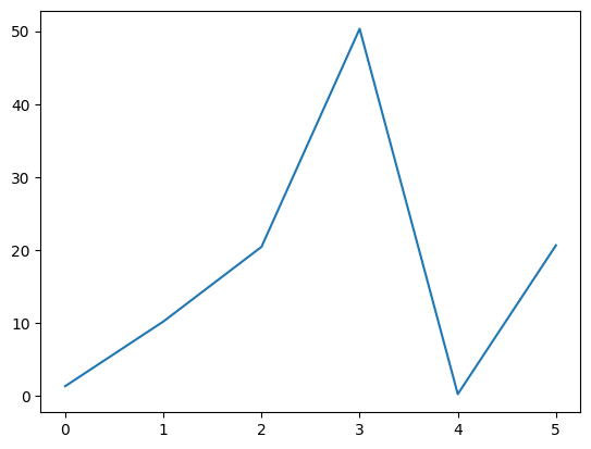
df2["Value"].plot()
<Axes: >